Tutorial
Let’s learn DIDPPy using the traveling salesperson problem with time windows (TSPTW) as an example.
TSPTW
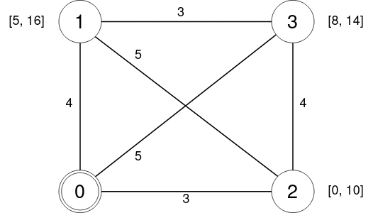
In TSPTW, we are given a set of locations \(N = \{ 0, ..., n-1 \}\). The salesperson starts from the depot \(0\), visit each customer \(i \in \{ 1, ..., n-1 \}\) exactly once, and returns to the depot. The traveling time from \(i\) to \(j\) is \(c_{ij}\). Each customer \(i\) must be visited within time window \([a_i, b_i]\), and the salesperson must wait until \(a_i\) if arriving at \(i\) before \(a_i\). The objective is to minimize the total travel time (not including the waiting time).
The following image is an example of TSPTW with four locations.
DP Formulation for TSPTW
In DP, using recursive equations, we decompose the problem into subproblems and describe the optimal value of the original problem using the values of the subproblems. Each problem is defined as a state, which is a tuple of variables that describe the problem. The value function \(V\) maps a state to the optimal value of the problem.
In TSPTW, think about visiting customers one by one. If the salesperson visits \(j\) from the depot, the problem is reduced to visiting customers \(N \setminus \{ 0, j \}\) from location \(j\) at time \(\max \{ c_{0j}, a_j \}\). Therefore, we can define a subproblem using the following three variables:
\(U \subseteq N\) : the set of unvisited customers.
\(i \in N\) : the current location.
\(t\) : the current time.
In general, when customer \(j \in U\) is visited from location \(i\) at time \(t\), the problem is reduced to visiting customers \(U \setminus \{ j \}\) from location \(j\) at time \(\max \{ t + c_{ij}, a_j \}\). To visit customer \(j\), the salesperson must arrive before \(b_j\), i.e., \(t + c_{ij} \leq b_j\). When all customers are visited, the salesperson must return to the depot from location \(i\). Overall, we get the following DP formulation:
In the first line, if there is no \(j \in U\) with \(t + c_{ij} \leq b_j\) while \(U \neq \emptyset\), we assume that \(V(U, i, t) = \min_{j \in \emptyset} c_{ij} + V(U \setminus \{ j \},j, \max \{ t + c_{ij}, a_j \}) = \infty\) because it takes the minimum over the empty set, and the subproblem does not have a solution.
We call the state \((N \setminus \{ 0 \}, 0, 0)\), which corresponds to the original problem, the target state.
This DP formulation is based on Dumas et al. [1].
Modeling in DIDPPy
Now, let’s model the above DP formulation in DIDPPy. Assume that the data is given. First, start with importing DIDPPy and creating the model.
import didppy as dp

# Number of locations
n = 4
# Ready time
a = [0, 5, 0, 8]
# Due time
b = [100, 16, 10, 14]
# Travel time
c = [
    [0, 3, 4, 5],
    [3, 0, 5, 4],
    [4, 5, 0, 3],
    [5, 4, 3, 0],
]

model = dp.Model(maximize=False, float_cost=False)
Because the objective is to minimize the total travel time, we set maximize=False.
We assume that the travel time is an integer, so we set float_cost=False.
Actually, maximize=False and float_cost=False are the default values, so we can omit them.
Object Types
First, we define an object type, which represents the type of objects that are used in the model. In TSPTW, customers are objects with the same object type.
customer = model.add_object_type(number=n)
When defining an object type, we need to specify the number of objects. If the number of objects is \(n\), the objects are indexed from \(0\) to \(n-1\) (not \(1\) to \(n\)) in DIDPPy. Object types are sometimes required to define a state, as explained later.
State Variables
A state of a problem is defined by state variables. There are four types of state variables:
SetVar: a set of the indices of objects associated with an object type.ElementVar: the index of an object associated with an object type.IntVar: an integer.FloatVar: a continuous value.
In TSPTW, \(U\) is a SetVar, \(i\) is an ElementVar, and \(t\) is an IntVar.
# U
unvisited = model.add_set_var(object_type=customer, target=list(range(1, n)))
# i
location = model.add_element_var(object_type=customer, target=0)
# t
time = model.add_int_var(target=0)
While \(i\) is an integer, we define it as an ElementVar as it represents an element in the set \(N\).
There are some practical differences between ElementVar and IntVar:
ElementVaris nonnegative.ElementVarcan be used to describe changes and conditions onSetVar.ElementVarcan be used to access a value of a table (explained later).
The value of an element variable should be an integer between 0 and n - 1 as it represents an element in the set \(N\).
However, you may want to make it larger than n - 1 for some cases (explained later).
In fact, you can increase its value to an arbitrary large number.
While we use the integer cost and an integer variable for \(t\), we can use the float cost and a float variable for \(t\) by using add_float_var() if we want to use continuous travel time.
The value of SetVar is a set of elements in \(N\).
Because the object type of unvisited is customer, which has n objects, unvisited can contain 0 to n - 1 (not 1 to n).
State variables are defined with their target values, values in the target state.
The objective of the DP model is to compute the value of the target state, i.e., \(U = N \setminus \{ 0 \}\), \(i = 0\), and \(t = 0\).
The target value of an SetVar can be a list or a set in Python.
In addition, we can initialize it using SetConst, which is created by create_set_const().
Tables of Constants
In TSPTW, \(a_i\), \(b_i\), and \(c_{ij}\) are constants depending on customers. In DIDPPy, such constants are defined as tables.
ready_time = model.add_int_table(a)
due_time = model.add_int_table(b)
travel_time = model.add_int_table(c)
By passing a nested list of int to add_int_table(), we can create up to a three-dimensional int table.
For tables more than three-dimensional, we can pass a dict in Python with specifying the default value used when an index is not included in the dict.
See add_int_table() for more details.
We can add different types of tables using the following functions:
In the case of add_set_table(), we can pass a list (or a dict) of list or set in Python with specifying the object type.
See add_set_table() and an advanced tutorial for more details.
The benefit of defining a table is that we can access its value using state variables as indices, as explained later.
Transitions
The recursive equation of the DP model is defined by transitions. A transition transforms the state on the left-hand side into the state on the right-hand side.
In TSPTW, we have the following recursive equation:
In DIDPPy, it is represented by a set of transitions.
for j in range(1, n):
    visit = dp.Transition(
        name="visit {}".format(j),
        cost=travel_time[location, j] + dp.IntExpr.state_cost(),
        preconditions=[
            unvisited.contains(j),
            time + travel_time[location, j] <= due_time[j]
        ],
        effects=[
            (unvisited, unvisited.remove(j)),
            (location, j),
            (time, dp.max(time + travel_time[location, j], ready_time[j]))
        ],
    )
    model.add_transition(visit)
The cost expression cost defines how the value of the left-hand side state, \(V(U, i, t)\), is computed based on the value of the right-hand side state, \(V(U \setminus \{ j \}, j, \max\{ t + c_{ij}, a_j \})\), represented by didppy.IntExpr.state_cost().
In the case of the continuous cost, we can use didppy.FloatExpr.state_cost().
We can use the values of state variables in the left-hand side state in cost, preconditions, and effects.
For example, location corresponds to \(i\) in \(V(U, i, t)\), so travel_time[location, j] corresponds to \(c_{ij}\).
Because location is a state variable, travel_time[location, j] is not just an int but an expression (IntExpr), whose value is determined given a state inside the solver.
Therefore, we cannot use c[location][j] and need to register c to the model as travel_time.
Also, travel_time[location, j] must be used instead of travel_time[location][j].
For ready_time and due_time, we can actually use a and b instead because they are not indexed by state variables.
When using a state variable or an expression as an index of a table, the value must not exceed the size of the table:
you need to make sure that j in travel_time[location, j] is not larger than n - 1.
If j > n - 1, the solver raises an error during solving.
However, sometimes, you may want to use j > n - 1 to represent a special case;
in the knapsack problem in the quick start, i becomes n in a state where all decisions are made.
Please make sure that you do not access any table using i in such a state.
Preconditions preconditions make sure that the transition is considered only when \(j \in U\) (unvisited.contains(j)) and \(t + c_{ij} \leq b_j\) (time + travel_time[location, j] <= due_time[j]).
The value of the left-hand side state is computed by taking the minimum (maximum for maximization) of cost over all transitions whose preconditions are satisfied by the state.
preconditions are defined by a list of Condition.
Effects effects describe how the right-hand side state is computed based on the left-hand side state.
Effects are described by a list of tuple of a state variable and its updated value described by an expression.
\(U \setminus \{ j \}\) :
unvisited.remove(j)(SetExpr).\(j\) :
j(automatically converted frominttoElementExpr).\(\max\{ t + c_{ij}, a_j \}\) :
dp.max(time + travel_time[location, j], ready_time[j])(IntExpr).
SetVar, SetExpr and SetConst have a similar interface as set in Python, e.g., they have methods contains(), add(), remove() which take an int, ElementVar, or ElementExpr as an argument.
We use didppy.max() instead of built-in max() to take the maximum of two IntExpr.
As in this example, some built-in functions are replaced by functions in DIDPPy to support expressions.
However, we can apply built-in sum(), abs(), and pow() to IntExpr.
The equation
is defined by another transition in a similar way.
return_to_depot = dp.Transition(
    name="return",
    cost=travel_time[location, 0] + dp.IntExpr.state_cost(),
    effects=[
        (location, 0),
        (time, time + travel_time[location, 0]),
    ],
    preconditions=[unvisited.is_empty(), location != 0]
)
model.add_transition(return_to_depot)
The effect on unvisited is not defined because it is not changed.
Once a transition is created, it is registered to a model by add_transition().
We can define a forced transition, by using forced=True in this function while it is not used in TSPTW.
A forced transition is useful to represent dominance relations between transitions in the DP model.
See an advanced tutorial for more details.
Base Cases
A base cases is a set of conditions to terminate the recursion. In our DP model,
is a base case.
In DIDPPy, a base case is defined by a list of Condition.
model.add_base_case([unvisited.is_empty(), location == 0])
When all conditions in a base case are satisfied, the value of the state is constant, and no further transitions are applied.
By default, the cost is assumed to be 0, but you can use an expression to compute the value given a state by using the argument cost in add_base_case().
We can define multiple independent base cases by calling add_base_case() multiple times, with different sets of conditions.
In that case, the value of a state is the minimum/maximum of the values of the satisfied base cases in minimization/maximization.
Solving the Model
Now, we have defined a DP model.
Let’s use the CABS solver to solve this model.
solver = dp.CABS(model, time_limit=10)
solution = solver.search()

print("Transitions to apply:")

for t in solution.transitions:
    print(t.name)

print("Cost: {}".format(solution.cost))
search() returns a Solution, from which we can extract the transitions that walk from the target state to a base case and the cost of the solution.
CABS is an anytime solver, which returns the best solution found within the time limit.
Instead of search(), we can use search_next(), which returns the next solution found.
CABS is complete, which means that it returns an optimal solution given enough time.
If we use time_limit=None (the default value), it continues to search until an optimal solution is found.
Whether the returned solution is optimal or not can be checked by didppy.Solution.is_optimal.
While CABS is usually the most efficient solver, it has some restrictions:
it solves the DP model as a path-finding problem in a graph, so it is only applicable to particular types of DP models.
Concretely, cost in all transitions must have either of the following structures:
w + dp.IntExpr.state_cost()w * dp.IntExpr.state_cost()dp.max(w, dp.IntExpr.state_cost())dp.min(w, dp.IntExpr.state_cost())
where w is an IntExpr independent of state_cost().
For float cost, we can use FloatExpr instead of IntExpr.
By default, CABS assumes that cost is the additive form.
For other types of cost, we need to tell it to the solver by using the argument f_operator, which takes either of didppy.FOperator.Plus, didppy.FOperator.Product, didppy.FOperator.Max, or didppy.FOperator.Min (Plus is the default).
An example is provided in an advanced tutorial.
If your problem does not fit into the above structure, you can use ForwardRecursion, which is the most generic but might be an inefficient solver.
For further details, see the guide for the solver selection as well as the API reference.
Improving the DP Model
So far, we defined the DP formulation for TSPTW, model it in DIDPPy, and solved the model using a solver. However, the formulation above is not efficient. Actually, we can improve the formulation by incorporating more information. Such information is unnecessary to define a problem but potentially helps a solver. We introduce three enhancements to the DP formulation.
Resource Variables
Consider two states \((U, i, t)\) and \((U, i, t')\) with \(t \leq t'\), which share the set of unvisited customers and the current location. In TSPTW, smaller \(t\) is always better, so \((U, i, t)\) leads to an equal or better solution than \((U, i, t')\). Therefore, we can introduce the following inequality:
With this information, a solver may not need to consider \((U, i, t')\) if it has already considered \((U, i, t)\). This dominance relation between states can be modeled by resource variables.
# U
unvisited = model.add_set_var(object_type=customer, target=list(range(1, n)))
# i
location = model.add_element_var(object_type=customer, target=0)
# t (resource variable)
time = model.add_int_resource_var(target=0, less_is_better=True)
Now, time is an IntResourceVar created by add_int_resource_var() instead of add_int_var(), with the preference less_is_better=True.
This means that if the other state variables have the same values, a state having a smaller value of time is better.
If less_is_better=False, a state having a larger value is better.
There are three types of resource variables in DIDPPy:
We have explained that \((U, i, t)\) dominates \((U, i, t')\) if \(t\) is less than or equal to \(t'\) since \((U, i, t)\) leads to an equal or better solution. In general, there is another requirement to define \(t\) as a resource variable: \((U, i, t)\) must lead to an equal or better solution that has equal or fewer transitions than \((U, i, t')\). In our DP model, since all solutions visit all customers and the depot, they have the same length, so we do not need to care about it.
State Constraints
In TSPTW, all customers must be visited before their deadlines. In a state \((U, i, t)\), if the salesperson cannot visit a customer \(j \in U\) before \(b_j\), the subproblem defined by this state does not have a solution. The earliest possible time to visit \(j\) is \(t + c_{ij}\) (we assume the triangle inequality, \(c_{ik} + c_{kj} \geq c_{ij}\)). Therefore, if \(t + c_{ij} > b_j\) for any \(j \in U\), we can conclude that \((U, i, t)\) does not have a solution. This inference is formulated as the following equation:
This equation is actually implied by our original DP formulation, but we need to perform multiple iterations of recursion to notice that: we can conclude \(V(U, i, t) = \infty\) only when \(\forall j \in U, t + c_{ij} > b_j\). The above equation makes it explicit, and we can immediately conclude that \(V(U, i, t) = \infty\) if the condition is satisfied.
In DyPDL, the above inference is modeled by state constraints, constraints that must be satisfied by all states. Because state constraints must be satisfied by all states, we use the negation of the condition, \(\forall j \in U, t + c_{ij} \leq b_j\), as state constraints:
for j in range(1, n):
    model.add_state_constr(
        ~unvisited.contains(j) | (time + travel_time[location, j] <= due_time[j])
    )
For each customer j, we define a disjunctive condition \(j \notin U \lor t + c_{ij} \leq b_j\).
~ is the negation operator of Condition, and | is the disjunction operator.
We can also use & for the conjunction.
We cannot use not, or, and and in Python because they are only applicable to bool in Python.
State constraints are different from preconditions of transitions. State constraints are evaluated each time a state is generated while preconditions are evaluated only when a transition is taken.
Dual Bounds
In model-based approaches such as mixed-integer programming (MIP), modeling the bounds on the objective function is commonly used to improve the efficiency of a solver. In the case of DIDP, we consider dual bounds on the value function \(V\) for a state \((U, i, t)\), which are lower bounds for minimization and upper bounds for maximization.
The lowest possible travel time to visit customer \(j\) is \(\min_{k \in N \setminus \{ j \}} c_{kj}\). Because we need to visit all customers in \(U\), the total travel time is at least
Furthermore, if the current location \(i\) is not the depot, we need to visit the depot. Therefore,
Similarly, we need to depart from each customer in \(U\) and the current location \(i\) if \(i\) is not the depot. Therefore,
The above bounds are modeled as follows:
min_to = model.add_int_table(
    [min(c[k][j] for k in range(n) if k != j) for j in range(n)]
)

model.add_dual_bound(min_to[unvisited] + (location != 0).if_then_else(min_to[0], 0))

min_from = model.add_int_table(
    [min(c[j][k] for k in range(n) if k != j) for j in range(n)]
)

model.add_dual_bound(
    min_from[unvisited] + (location != 0).if_then_else(min_from[location], 0)
)
We first register \(\min\limits_{k \in N \setminus \{ j \}} c_{kj}\) to the model as a table min_to.
min_to[unvisited] represents \(\sum\limits_{j \in U} \min\limits_{k \in N \setminus \{ j \}} c_{kj}\), i.e., the sum of values in min_to for customers in unvisited.
Similarly, min_to.product(unvisited) min_to.max(unvisited), and min_to.min(unvisited) can be used to take the product, maximum, and minimum.
We can do the same for tables with more than one dimension.
For example, if table is a two-dimensional table, table[unvisited, unvisited] takes the sum over all pairs of customers in unvisited, and table[unvisited, location] takes the sum of table[i, location] where i iterates through customers in unvisited.
When the current location is not the depot, i.e., location != 0, \(\min\limits_{k \in N \setminus \{ 0 \}} c_{k0}\) (min_to[0]) is added to the dual bound, which is done by if_then_else().
We repeat a similar procedure for the other dual bound.
Note that dual bounds in DyPDL represent the bounds on the value of the problem defined by the given state, so they are state-dependent. Dual bounds are not just bounds on the optimal value of the original problem, but they are used in each subproblem.
Defining a dual bound in DIDP is extremely important: a dual bound may significantly boost the performance of solvers. We strongly recommend defining a dual bound even if it is trivial, such as \(V(U, i, t) \geq 0\).
Full Formulation
Overall, our model is now as follows:
Note that in the second line, \(t + c_{ij} \leq b_j\) for \(j \in U\) is ensured by the first line.
Here is the full code for the DP model:
import didppy as dp

# Number of locations
n = 4
# Ready time
a = [0, 5, 0, 8]
# Due time
b = [100, 16, 10, 14]
# Travel time
c = [
    [0, 3, 4, 5],
    [3, 0, 5, 4],
    [4, 5, 0, 3],
    [5, 4, 3, 0],
]

model = dp.Model(maximize=False, float_cost=False)

customer = model.add_object_type(number=n)

# U
unvisited = model.add_set_var(object_type=customer, target=list(range(1, n)))
# i
location = model.add_element_var(object_type=customer, target=0)
# t (resource variable)
time = model.add_int_resource_var(target=0, less_is_better=True)

ready_time = model.add_int_table(a)
due_time = model.add_int_table(b)
travel_time = model.add_int_table(c)

for j in range(1, n):
    visit = dp.Transition(
        name="visit {}".format(j),
        cost=travel_time[location, j] + dp.IntExpr.state_cost(),
        preconditions=[unvisited.contains(j)],
        effects=[
            (unvisited, unvisited.remove(j)),
            (location, j),
            (time, dp.max(time + travel_time[location, j], ready_time[j])),
        ],
    )
    model.add_transition(visit)

return_to_depot = dp.Transition(
    name="return",
    cost=travel_time[location, 0] + dp.IntExpr.state_cost(),
    effects=[
        (location, 0),
        (time, time + travel_time[location, 0]),
    ],
    preconditions=[unvisited.is_empty(), location != 0],
)
model.add_transition(return_to_depot)

model.add_base_case([unvisited.is_empty(), location == 0])

for j in range(1, n):
    model.add_state_constr(
        ~unvisited.contains(j) | (time + travel_time[location, j] <= due_time[j])
    )

min_to = model.add_int_table(
    [min(c[k][j] for k in range(n) if k != j) for j in range(n)]
)

model.add_dual_bound(min_to[unvisited] + (location != 0).if_then_else(min_to[0], 0))

min_from = model.add_int_table(
    [min(c[j][k] for k in range(n) if k != j) for j in range(n)]
)

model.add_dual_bound(
    min_from[unvisited] + (location != 0).if_then_else(min_from[location], 0)
)

solver = dp.CABS(model)
solution = solver.search()

print("Transitions to apply:")

for t in solution.transitions:
    print(t.name)

print("Cost: {}".format(solution.cost))
Next Steps
Congratulations! You have finished the tutorial.
We covered fundamental concepts of DIDP modeling and advanced techniques to improve the performance of the model.
Several features that did not appear in the DP model for TSPTW are covered in the advanced tutorials.
More examples are provided in our repository as Jupyter notebooks.
The API reference describes each class and function in detail.
If your model does not work as expected, the debugging guide might help you.
If you want to know the algorithms used in the solvers, we recommend reading Kuroiwa and Beck [2].
Our papers on which DIDPPy is based are listed on this page.